
Introduction
MFT Reader is a forensic GUI application that analyzes the NTFS Master File Table ($MFT) and USN Change Journal ($J) to surface suspicious filesystem activity. This article focuses on functionality that directly supports the forensic analyst: triage and prioritization, timeline reconstruction, evidence review, cross-tab workflow, and how to use each feature to accelerate investigations when process context is missing.
Why It Works Without Process Data: Filesystem-Only Detection
The application operates under a strict constraint: no process context. There are no PIDs, command lines, or parent-child process relationships. All detection is based purely on what happened to files on disk—when they were created, written, renamed, overwritten, and deleted.
The USN (Update Sequence Number) is used as the primary ordering key everywhere. Timestamps can be modified by an attacker; USN is a kernel-managed monotonic counter that cannot be altered from userspace. The application never relies on timestamp ordering alone for critical logic.
Where to Start: Triage and Prioritization
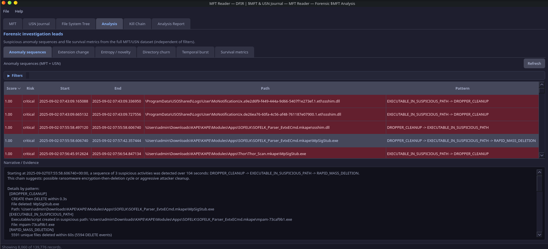
When you load $MFT and $J and click Refresh in the Anomaly sequences tab, the application returns attack chains (linked findings) sorted by chain score descending. The analyst should start at the top of this list—the highest-scoring chain represents the most suspicious coordinated activity. Each chain has a human-readable narrative (e.g., “malware deployment with post-execution self-deletion”, “possible ransomware encryption-then-deletion cycle”) that gives you a working hypothesis; the constituent events and evidence list provide the supporting detail.
Severity thresholds help you prioritize:
- 0.80–1.0 (Critical) — Investigate immediately; high confidence malicious
- 0.60–0.79 (High) — Strong indicators; analyst review required
- 0.40–0.59 (Medium) — Suspicious but may be legitimate; context needed
- 0.00–0.39 (Low) — Weak signal; flag for awareness
In the MFT tab and File System Tree, rows are risk-highlighted (Critical / High / Medium) for timestomping, executables in suspicious paths (Temp, Public, $Recycle.Bin, Startup, Tasks), and high sequence numbers. You can sort by any column and quickly spot the most relevant records without applying filters first.
Scenario: You have a disk image from a suspected compromise. You load $MFT and $J, open the Analysis tab, and click Refresh on Anomaly sequences. The top row is an attack chain (score 0.92) with narrative “malware deployment with post-execution self-deletion.” You start there: select the row, read the evidence panel, then jump to the MFT records for the flagged paths to correlate with other artifacts.
How Anomaly Detection Works: Patterns, Scores, and Chains
The application runs seven pattern detectors on the normalized event stream. Each detector operates on one of: events_by_ref, events_by_parent, or the full event_stream.
Pattern Detectors
| Pattern | Input | Logic | Base Score |
|---|---|---|---|
| DROPPER_CLEANUP | events_by_ref | CREATE + DELETE on same file within 300s; suspicious extension + path | 0.75 |
| MASQUERADE_RENAME | events_by_ref | RENAME_OLD_NAME → RENAME_NEW_NAME to system binary name (svchost, explorer, etc.) from random/temp source | 0.90 |
| STAGED_DROPPER | events_by_parent | 3+ CREATEs in same directory within 120s; suspicious or archive extensions; suspicious path | 0.70 |
| OVERWRITE_THEN_DELETE | events_by_ref | OVERWRITE then DELETE within 30s (anti-forensic wipe) | 0.80 |
| RAPID_MASS_DELETION | event_stream | 20+ DELETEs within 60s (ransomware or cleanup) | 0.85 |
| EXECUTABLE_IN_SUSPICIOUS_PATH | event_stream | CREATE with suspicious extension in suspicious path | 0.60 |
| TIMESTOMP_WITH_WRITE | events_by_ref | WRITE then METADATA within 5s + timestomp detected | 0.85 |
Composite Scoring
Each finding receives a composite_score = min(base_score + sum(modifiers), 1.0). Modifiers include:
- Timestomp detected (+0.15): |si_created − fn_created| > 2 seconds, or si_created has zero microseconds
- is_deleted_record (+0.10): MFT slot no longer in use
- Script extension (+0.10): .ps1, .vbs, .js, .bat
- Pattern-specific modifiers (e.g., duration < 30s for DROPPER_CLEANUP, burst > 10 files for STAGED_DROPPER)
Attack Chain Linking
Findings that are temporally and spatially related are linked into AttackChain objects. Two findings are linked if:
- Temporal proximity: Time gap between end of A and start of B ≤ 300 seconds
- Spatial relationship: Same parent directory path, or shared file_ref across events
Chain score = min(average(finding scores) × 1.3, 1.0). A human-readable narrative is generated (e.g., “malware deployment with post-execution self-deletion”, “possible ransomware encryption-then-deletion cycle”).
Reviewing Evidence and Drilling Down into Findings
Selecting a row in the Anomaly sequences table populates the Narrative / Evidence panel below. For an attack chain, you see the full narrative and the list of linked findings; for a single finding, you see the evidence list—short, human-readable bullets explaining why it was flagged (e.g., “CREATE then DELETE within 45.2s”, “File deleted: payload.exe”, “Path: C:\Users\…\AppData\Local\Temp\…”). This gives the analyst a clear audit trail from finding to underlying events.
In Directory churn, double-clicking a row opens a dialog listing every file in that burst, with extension and risk highlights (Executable?, Persistence path?). You can quickly verify whether a burst is benign (e.g., installer extraction) or suspicious (mix of executables and scripts in Temp).
Analysis reports use the full loaded dataset—they are independent of the MFT and USN tab filters. So even if you narrow the MFT view to a time window or path, when you switch to Analysis and click Refresh, you get reports over the complete $MFT and $J. That way you do not miss anomalies outside the current filter.
Scenario: You select a DROPPER_CLEANUP finding; the evidence panel shows “CREATE then DELETE within 12.3s”, “File deleted: update.exe”, “Path: C:\Users\…\AppData\Local\Temp\…”. You note the path and MFT #, then switch to the MFT tab and search for that record. In Directory churn you see a burst in the same Temp folder; you double-click the row and the dialog lists update.exe plus several .dll and .dat files—consistent with a dropper unpacking and then deleting itself.
Reports That Surface Suspicious Patterns: Entropy, Churn, and Bursts
Filename Entropy (Shannon)
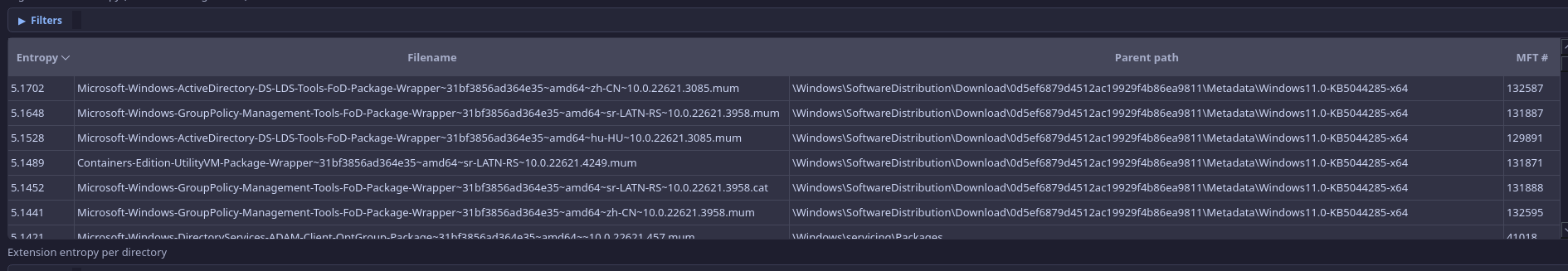
For the analyst, high-entropy filenames often indicate machine-generated or random names used by malware or droppers; the report lists the top entries by entropy so you can quickly review the most suspicious names.
For each file, the application computes Shannon entropy of the filename: H = −Σ p(c) log₂(p(c)) over distinct characters. High entropy indicates random-looking or machine-generated names (e.g., malware droppers). Results are sorted by entropy descending.
Scenario: You open the Filename entropy report and the top entries include names like a8f3c2d1e4b9.exe and tmp7a2f91.tmp in user Temp folders. You add a path filter containing “Temp” and review the list—several high-entropy .exe and .dll names in the same directory suggest a dropper or packed payload; you cross-check with Anomaly sequences and Directory churn for the same paths.
Extension Entropy per Directory
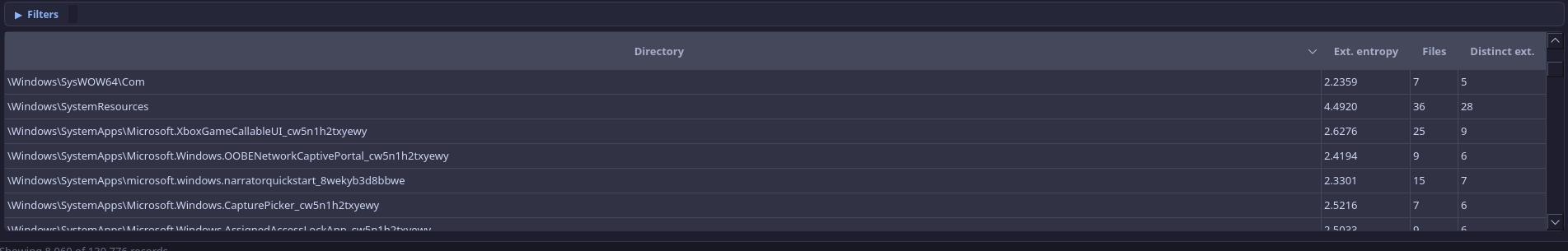
For each directory, the application computes Shannon entropy of the distribution of file extensions among its direct children. High entropy = many different extension types; low entropy = few types (e.g., all .txt). Unusual diversity may warrant investigation.
Scenario: A user folder that should mostly contain documents (.docx, .pdf) appears at the top of the Extension entropy report with high entropy and many distinct extensions (.exe, .dll, .ps1, .zip, .dat). You open that path in the File System Tree and MFT tab to see what was created when—it may indicate a toolkit or staged payloads in a non-standard location.
Directory Churn
For the analyst, this answers: “Where did many files appear in a short time?”—typical of dropper extraction, payload staging, or bulk persistence. You set the time window (e.g. 120s) and minimum file count; the table shows directory, burst size, first/last file, and flags (Executable?, Persistence path?). Double-click a row to see every file in that burst.
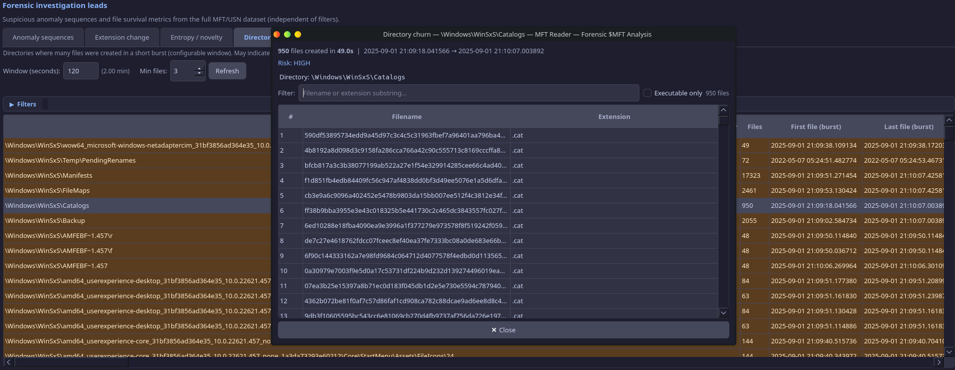
Uses a sliding-window algorithm per parent directory. MFT and USN data are merged and deduplicated by (parent_directory, filename)—when both exist, the USN timestamp wins (real event time). For each directory, the algorithm finds bursts of ≥ min_files unique filenames within a configurable window (default 120 seconds). Directories in persistence paths (Startup, Tasks, Temp) or containing executables are scored higher (critical/high risk).
Scenario: You are looking for dropper or extraction activity. You set Directory churn window to 60 seconds and Min files to 5, then Refresh. A row shows C:\Users\…\AppData\Local\Temp with 12 files in 45 seconds, Executable? yes, Persistence? no. You double-click the row: the dialog lists an .exe, two .dlls, and several .dat/.tmp files. You add the .exe to the Kill Chain (Installation or Delivery) and note the path for your report.
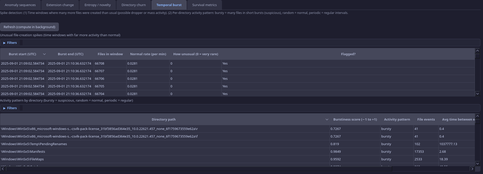
Temporal Burst (Poisson + Burstiness)
Two complementary views:
- Poisson anomaly: Baseline λ = mean events per minute over the timeline. For each sliding window, compute observed count k and P(X ≥ k) under Poisson(λ). If P(X ≥ k) < 0.001 → anomaly (burst). Highlights time windows where file creation spikes far exceed the expected rate.
- Burstiness B: Per directory, compute inter-arrival times between events → μ (mean), σ (std). B = (σ − μ) / (σ + μ). B ≈ +1 → bursty (malware-like); B ≈ −1 → periodic; B ≈ 0 → random.
This report runs in a background thread because it iterates over the full merged MFT+USN event stream with sliding windows.
Scenario: You run the Temporal burst report to find when file creation spiked. The Poisson view shows a 60-second window with 80+ creations (P(X≥k) < 0.001) at 14:23; the Burstiness view shows a Temp directory with “bursty” activity. You set the MFT time anchor to 14:23 ± 120 seconds and review what was created in that window—you find the initial drop and several follow-up writes that align with the burst.
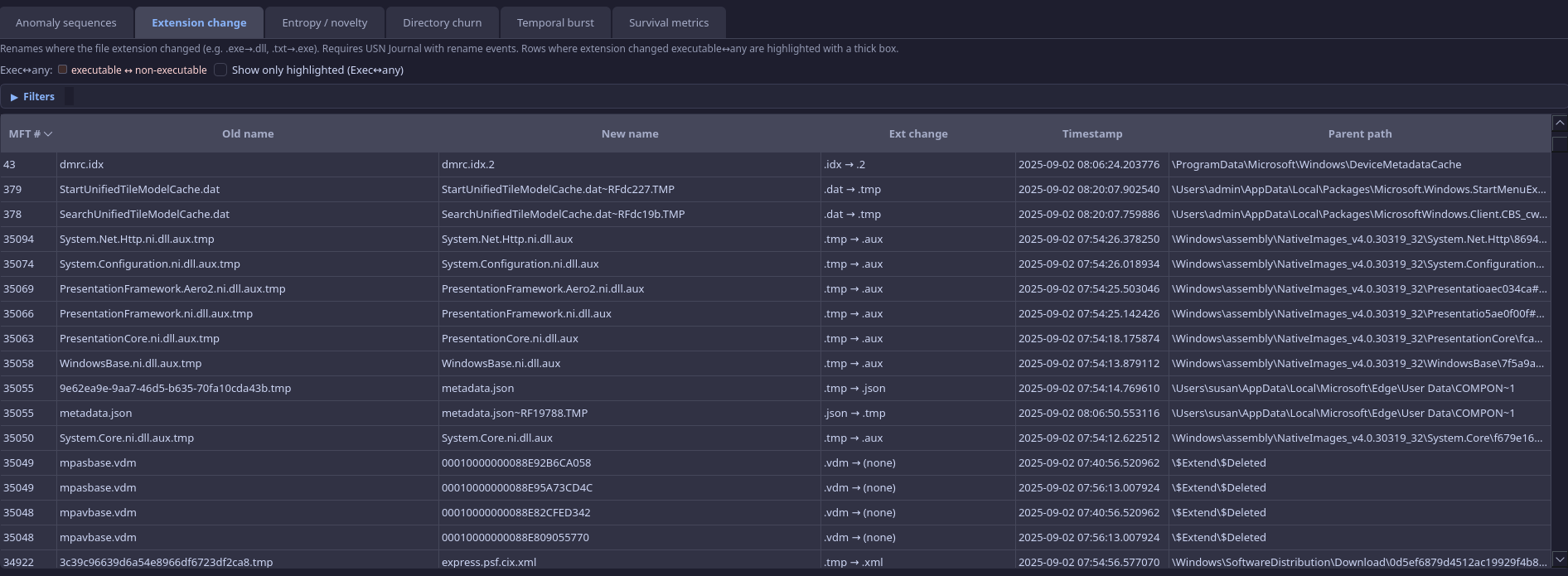
Finding Disguised Executables: Extension Change Detection
For the analyst, this report answers: “Where did something rename to look like a different file type?”—e.g. .txt→.exe or .doc→.exe. Rows where the extension changed between executable and non-executable are highlighted; you can filter to “Show only highlighted (Exec↔any)” to focus on the most relevant renames.
Uses USN Journal records with RENAME_OLD_NAME and RENAME_NEW_NAME. For each file_ref, the application pairs each RENAME_OLD_NAME with the next RENAME_NEW_NAME (by timestamp). If the extension (suffix after last dot) differs, the rename is reported—e.g., .txt→.exe for disguised executables.
Scenario: You suspect a phishing payload was delivered as a “document” and then renamed to run. In the Extension change report you enable “Show only highlighted (Exec↔any).” You see invoice.pdf → invoice.exe in a user Downloads folder. You note the MFT # and timestamp, add the file to the Kill Chain (Delivery or Exploitation), and correlate with Survival metrics to see if it was deleted shortly after (dropper behavior).
Which Deleted Files Lived Only a Short Time? Survival Metrics
For the analyst, this answers: “Which deleted files lived only a short time?”—a strong signal for droppers (create → execute → delete) or staged payloads. The table is sorted by time-to-delete ascending so the shortest-lived files appear first; the histogram groups short-lived files (<5 min) into buckets for a quick overview.
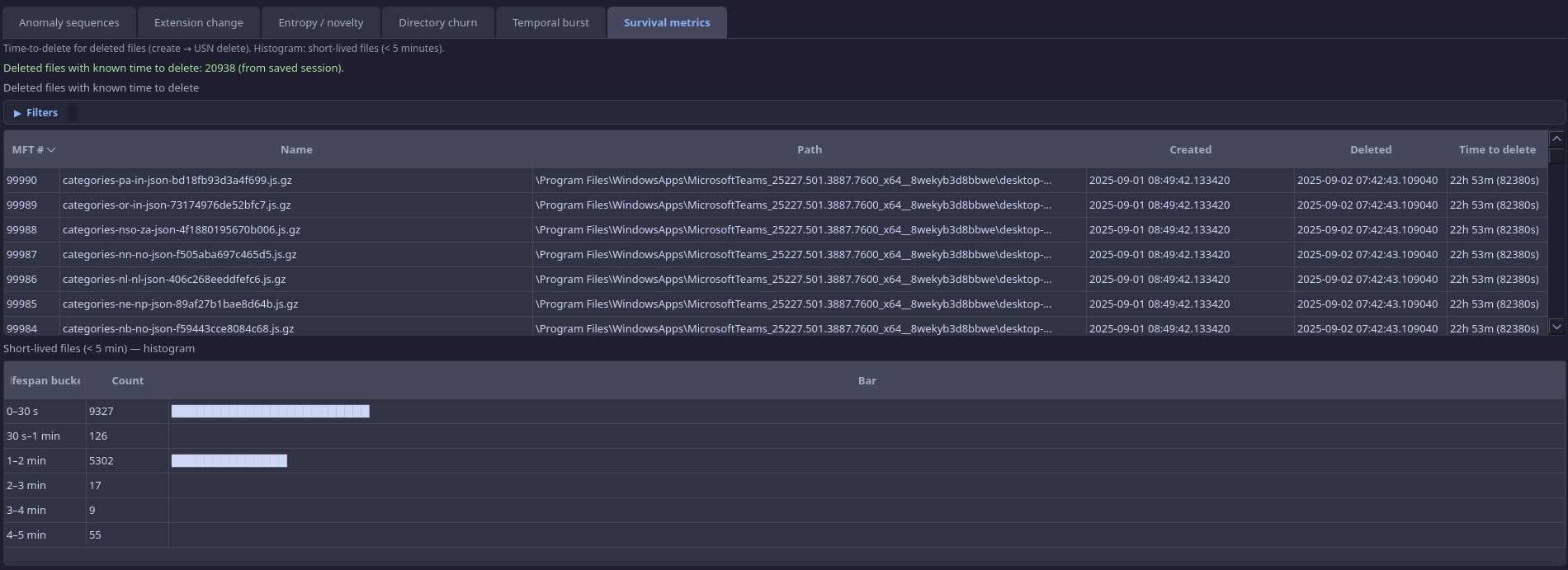
Requires the USN Journal. The application performs lifecycle reconstruction by file_ref (which includes sequence number, so it tracks a specific file instance):
- For each file_ref, track earliest FILE_CREATE timestamp and latest FILE_DELETE timestamp
- Compute time-to-delete = delete_ts − create_ts
- Build a table of deleted files with known lifetime, sorted by time-to-delete ascending
- Build a histogram of short-lived files (< 5 min) in buckets: 0–30s, 30s–1min, 1–2min, 2–3min, 3–4min, 4–5min
Short-lived files may indicate staged payloads or dropper self-deletion.
Scenario: You want to find executables that ran and then deleted themselves. In Survival metrics the table is sorted by time-to-delete ascending. The first few rows show .exe and .ps1 files in Temp with lifetimes of 8s, 12s, 30s. You cross-reference with Anomaly sequences—one of them is in a DROPPER_CLEANUP finding. The histogram shows a spike in the 0–30s bucket; you document that as evidence of short-lived staged payloads.
Where to Carve for Deleted Content: Sequence Gap Report
For the analyst, this helps prioritize where to look for deleted content: high sequence means the slot has been reused many times (create/delete cycles), so unallocated space or carving in that directory may yield previously deleted files.
MFT record slots are reused. Each reuse increments the sequence number. High sequence = this slot has been a “graveyard” for many deleted files. The application flags records with sequence ≥ 5 (configurable), sorted by sequence descending. Useful for identifying directories where deeper carving may recover deleted content.
Scenario: You are looking for evidence of deleted malware in a user profile. The Sequence gap report shows several records in C:\Users\…\AppData\Local\Temp with sequence 8–12. You note those paths and MFT record numbers; later you run a file carver or inspect unallocated space in that directory to try to recover earlier versions of deleted files that occupied those slots.
Spotting Backdated Timestamps: Timestomp Detection
For the analyst, timestomp detection highlights files whose timestamps were likely manipulated (e.g. to hide when a file was really created). It is used as a modifier across the app—it raises the score of anomaly findings and appears as a risk hint in the MFT table and File System Tree; it is not a standalone report.
A file is considered timestamp-suspicious if either:
- Condition 1: |si_created − fn_created| > 2 seconds. Attackers often modify $STANDARD_INFORMATION but leave $FILE_NAME intact.
- Condition 2: si_created.microsecond == 0. Legitimate Windows timestamps have non-zero sub-second precision; zero indicates manual setting.
Timestomp alone is not a finding—it is a modifier that elevates the score of any pattern where it is detected.
Scenario: A finding in Anomaly sequences has an elevated score in part because “timestomp detected” was applied. You open the MFT record for that file: the $STANDARD_INFORMATION created time is months ago, while the $FILE_NAME created time (and USN) show it was created during the incident window. You document that the file was backdated to blend in with legitimate software—useful for establishing intent in your report.
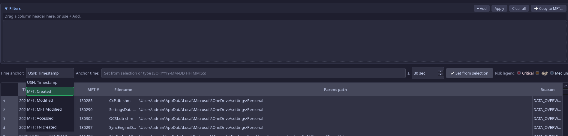
Focusing Your View: Filters, Time Anchor, and Copying to USN
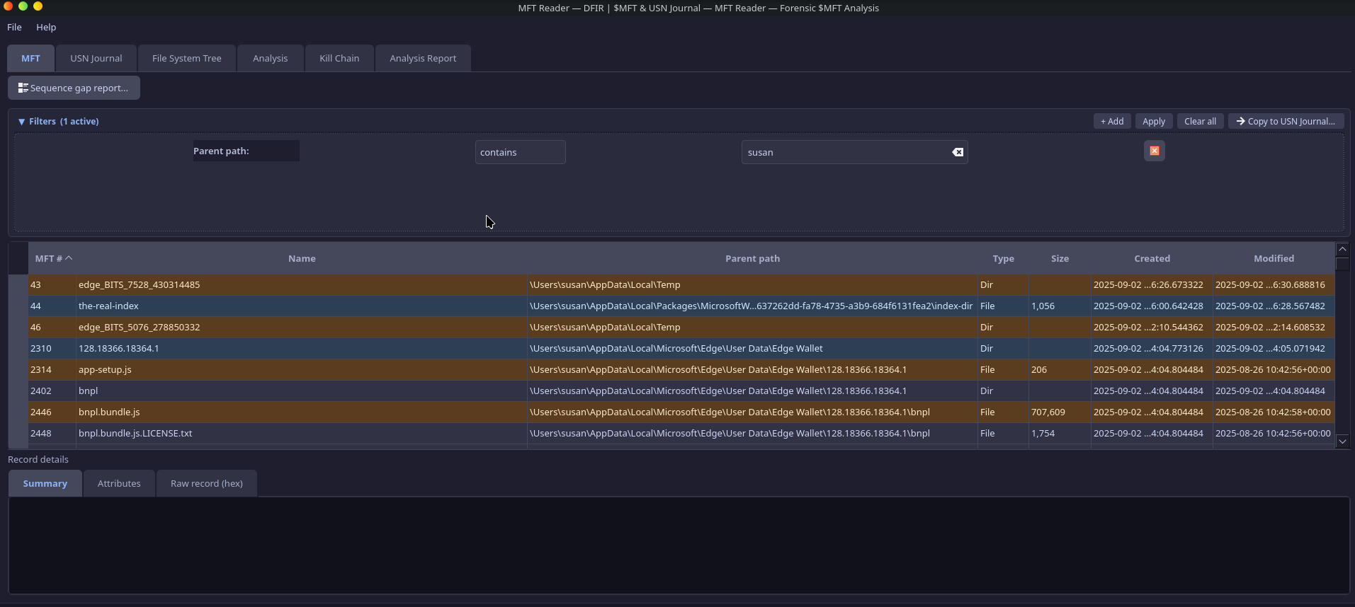
Compound filters: Drag column headers into the filter panel; criteria are ANDed. Operators: contains, equals, starts with, ends with, glob (* ?) for text; equals, not equals, <, >, <=, >= for numbers. This lets the analyst narrow the MFT or USN view by path, extension, timestamp, or MFT # without leaving the tab.
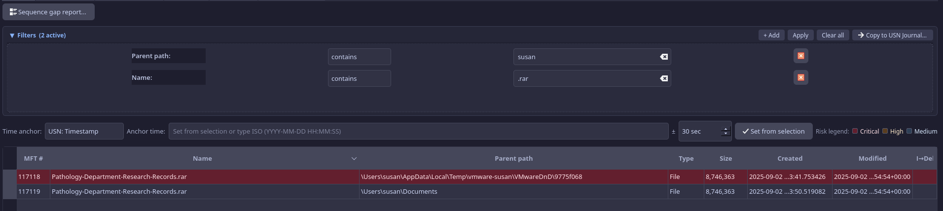
Time anchor: Restrict records to ±N seconds around an anchor timestamp. When you have a known incident time (e.g., from a log or alert), set the anchor to that time and adjust the ± seconds (e.g., ±300). Only records inside that window are shown—ideal for “what changed around this moment?” You can Set anchor from selection: select a row in the MFT or USN table whose timestamp you want to use, then click the button; the anchor is filled from that row’s time column.
Copy filters: The same compound filter panel and time anchor are available on both the MFT and USN Journal tabs. You can copy filters from MFT to USN (or vice versa) so that both views show the same logical slice of data. That keeps your investigation context consistent when you correlate MFT records with journal events.
Risk highlighting: Rows are colored by Critical / High / Medium based on timestomping, executables in suspicious paths, and high sequence numbers, so high-value records stand out even in large tables.
Scenario: Your SIEM alert says the host was compromised at 2024-06-15 14:22:00 UTC. You load the image’s $MFT and $J in MFT Reader. You set the time anchor to 2024-06-15 14:22:00 and ±300 seconds. The MFT tab now shows only records in that 10-minute window. You apply a path filter “contains \Temp” to focus on Temp activity. You copy filters to the USN Journal tab so both tabs show the same slice; you compare MFT records with USN events (creates, renames, deletes) to build a precise sequence of what appeared and disappeared around the incident time.
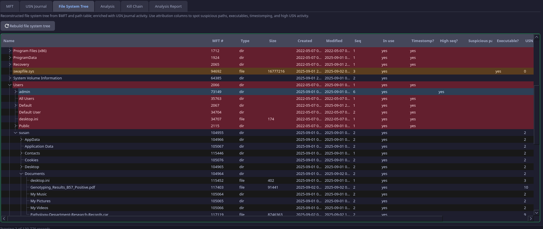
Browsing the Disk: File System Tree and Forensic Hints
The File System Tree tab reconstructs the directory hierarchy from the MFT. It loads lazily (expand a folder to load its children), so you can navigate large volumes without loading everything at once. Each node can show forensic hints:
- Timestomp? — $STANDARD_INFORMATION vs $FILE_NAME creation time disagreement
- High seq? — High sequence number (reused MFT slot; possible deleted-file graveyard)
- Suspicious path? — Path matches Temp, Public, $Recycle.Bin, Startup, Tasks, etc.
- Executable? — File has an executable extension (.exe, .dll, .ps1, etc.)
These hints help the analyst scan the tree for anomalies without opening every file. Combined with the MFT table (sortable, filterable), the tree supports both path-centric and record-centric investigation.
Scenario: You need to quickly check whether anything suspicious exists under a user’s AppData. You open the File System Tree and expand C:\Users\…\AppData\Local. One subfolder shows “Suspicious path? Executable?” on a node. You expand it and see an .exe with “Timestomp?” You right-click that file, add it to the Kill Chain (e.g. Installation), then jump to the MFT row to capture full path and timestamps for your timeline.
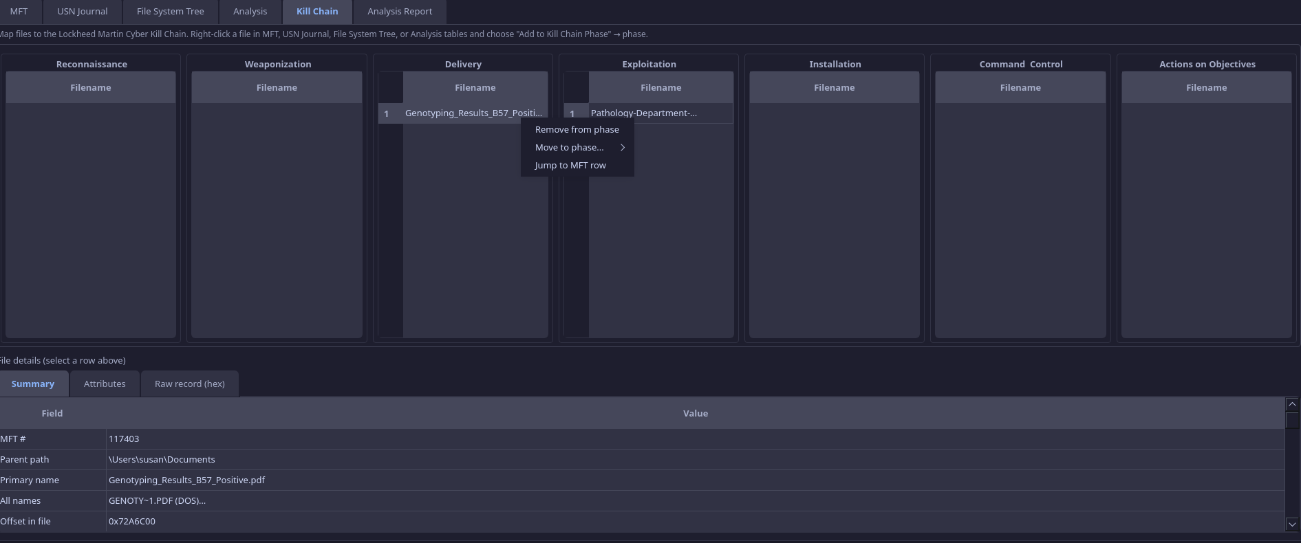
Mapping Artifacts to the Kill Chain
The Kill Chain tab maps files to the Lockheed Martin Cyber Kill Chain phases: Reconnaissance, Weaponization, Delivery, Exploitation, Installation, Command & Control, Actions on Objectives. From the MFT, USN Journal, File System Tree, or from Analysis sub-tabs that show MFT # (Extension change, Filename entropy, Survival metrics), you can right-click a row and choose Add to Kill Chain Phase → select a phase. The file is added to that phase in the Kill Chain tab. There you can select a row to see full file details, right-click to remove it, move it to another phase, or jump to the MFT row. Kill chain assignments are saved and restored with the session.
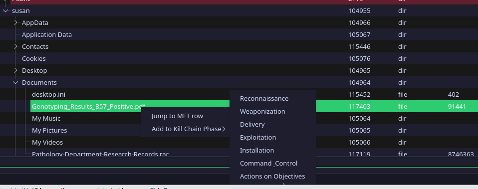
This helps the analyst build a structured view of the attack: which artifacts belong to delivery vs installation vs C2, and to document the lifecycle for reports or handover.
Scenario: You have identified a dropped loader (from Anomaly sequences), a renamed document (from Extension change), and a script in Startup (from Directory churn). You right-click each in their respective tables and add them to Kill Chain phases: the loader to Installation, the document to Delivery, the script to Installation or C2. In the Kill Chain tab you review the list by phase, move one file to a different phase if needed, and use “Jump to MFT row” to double-check details. When you save the session, the Kill Chain assignments are preserved for the next session.
Saving Your Work: Session, CSV Export, and Report
Save session (Ctrl+S) persists the paths to $MFT and $J, filter state, time anchor, column visibility, and Kill Chain assignments to a .mftsession file (JSON). Load session (Ctrl+L) restores everything so you can resume an investigation without re-opening dialogs or re-applying filters.
Export CSV exports the currently visible/filtered MFT table rows to a CSV file. Only rows that pass the current MFT tab filters and time anchor are included. The analyst can feed this into timeline tools (e.g., Plaso, log2timeline), SIEM (Splunk, ELK), or spreadsheets for further analysis or reporting.
The Analysis tab includes a Refresh report button that regenerates a text summary of the current Analysis and Kill Chain state—useful for pasting into case notes or appendices.
Scenario: At the end of the day you have applied time anchor (incident window), identified several findings, and populated the Kill Chain. You save the session (Ctrl+S) so tomorrow you can load it (Ctrl+L) and continue without re-opening $MFT/$J or re-applying filters. You export CSV with the current MFT filter (e.g. incident window + path contains Temp) and import that CSV into your timeline tool or SIEM to correlate with network and process data. You click Refresh report and paste the summary into your case notes as an appendix of key MFT/USN findings.
See It in Action: Three Real Case Studies
The following cases illustrate how an analyst uses MFT Reader’s functions in a real investigation. Names and paths are representative; the workflow applies to any similar incident.
Case 1: Phishing Dropper (Document → Executable → Self-Delete)
Context: A user reported a suspicious email; the host was isolated and imaged. The email arrived at 09:14; the user opened the attachment at 09:16. You have $MFT and $J from the image. No process memory or full event logs are available.
How the analyst uses the tool:
- Time anchor — You set the anchor to 09:16 and ±600 seconds. The MFT and USN tabs now show only activity in that 20-minute window. You copy filters to the USN tab so both views stay in sync.
- Anomaly sequences — You open Analysis → Anomaly sequences → Refresh. The top finding is an attack chain (score 0.88): “malware deployment with post-execution self-deletion.” The evidence panel shows a file created in
C:\Users\jdoe\AppData\Local\Temp, then deleted within 18 seconds. You note the path and MFT #. - Extension change — In the Extension change report you enable “Show only highlighted (Exec↔any).” You see
Q2_Report.docx→Q2_Report.exein the user’s Downloads folder at 09:16:42. This matches the phishing lure; the rename is the moment the “document” became an executable. - Survival metrics — You switch to Survival metrics. The table (sorted by time-to-delete) shows an .exe in Temp with a lifetime of 18 seconds. The histogram shows one file in the 0–30s bucket. You document: “Dropper lived 18s; create → execute → self-delete.”
- Directory churn — In Directory churn you see a burst in the same Temp path: 4 files in 12 seconds (the .exe plus 3 others). You double-click the row: the dialog lists the .exe and three .dat/.tmp files—likely the dropper and unpacked payloads before deletion.
- Kill Chain — You right-click the renamed file in Extension change and add it to Delivery. You right-click the short-lived .exe in Survival metrics and add it to Installation. In the Kill Chain tab you now have a clear Delivery → Installation sequence for the report.
- Export & report — You export CSV (with time anchor and path filter on Temp/Downloads) and add it to your timeline. You click Refresh report and paste the summary into the case file.
Benefit: Without process or command-line data, you have reconstructed the delivery mechanism (renamed attachment), the execution location (Temp), the short-lived dropper, and the burst of related files—and mapped it to the Kill Chain. Time anchor and copy filters kept MFT and USN aligned; anomaly sequences gave you a single place to start.
Case 2: Ransomware (Mass Deletion and Overwrite-Then-Delete)
Context: A file server was hit; hundreds of files were encrypted and originals deleted. You have $MFT and $J from the server volume. You need to establish when the mass deletion started and which directories were hit first.
How the analyst uses the tool:
- Anomaly sequences — You load $MFT and $J and run Anomaly sequences → Refresh. You see a RAPID_MASS_DELETION finding (score 0.92): 140+ files deleted within 60 seconds, and an OVERWRITE_THEN_DELETE finding in a user share. The narrative suggests “possible ransomware encryption-then-deletion cycle.” You note the start and end timestamps of the finding.
- Time anchor — You set the anchor to the start time of the RAPID_MASS_DELETION finding and ±120 seconds. In the MFT tab you filter by path (e.g. the affected share). You see the wave of deletions in USN order; you copy filters to the USN tab to correlate.
- Temporal burst — You run the Temporal burst report (Refresh in background). The Poisson view shows an extreme spike in file activity in that same 2-minute window; the burstiness view shows “bursty” activity in the share path. You use this to document “abnormal creation/deletion spike consistent with encryption and deletion.”
- Survival metrics — Many deleted files now have time-to-delete in the table. You sort by time-to-delete ascending; a cluster of very short lifetimes (under 60s) in the share supports the “encrypt then delete original” pattern. The histogram shows a large count in the 0–30s and 30s–1min buckets.
- Sequence gap — You open the Sequence gap report. Several records in the affected share have high sequence numbers (8–15). You note those paths and MFT #s for your team: these slots are good candidates for carving or recovery attempts of pre-encryption content.
- File System Tree — You browse to the share in the File System Tree. Nodes show “High seq?” where slots were heavily reused. You use this to prioritize which folders to document for the recovery team.
- Export — You export CSV for the incident window (time anchor + path filter on the share) and feed it into the timeline to compare with backup and restore events.
Benefit: You have identified the mass-deletion window, linked it to overwrite-then-delete (anti-forensic wipe), used temporal burst to support the timeline, and used survival metrics and sequence gap to prioritize recovery and carving—all from $MFT and $J.
Case 3: Persistence and Timestomping (Startup Executable with Backdated Timestamps)
Context: During a compromise assessment you are reviewing a workstation image. You suspect a script or executable was placed in a startup or Tasks folder and that timestamps were altered to avoid detection.
How the analyst uses the tool:
- File System Tree — You open the File System Tree and expand
C:\Users\…\AppData\Roaming\Microsoft\Windows\Start Menu\Programs\Startup. One file shows Timestomp? and Executable?. You expand and note the filename; you right-click and add it to the Kill Chain (Installation) for later. - Risk highlighting (MFT tab) — In the MFT tab you sort by path and scroll to Startup and Tasks folders. Rows are risk-highlighted (Critical/High) for “executable in suspicious path” and “timestomp.” You identify two executables in Startup and one scheduled task script; one of them has a timestomp hint.
- Anomaly sequences — You run Anomaly sequences → Refresh. You see EXECUTABLE_IN_SUSPICIOUS_PATH for the Startup executable and TIMESTOMP_WITH_WRITE for the same file (write then metadata change within 5s, with SI vs FN delta). The evidence panel states the path and “timestomp detected.” You select the finding and read the narrative.
- Directory churn — You open Directory churn and set the window to 300 seconds, min files 2. You see a row for the Startup folder: 2 files in 10 seconds, Executable? yes, Persistence? yes. You double-click: the dialog lists the .exe and a .vbs. You document persistence mechanism (Startup + script).
- Timestomp (in context) — In the MFT tab you open the record for the timestomped file. The $STANDARD_INFORMATION created time is months in the past; the $FILE_NAME created time and USN timestamps place creation during the suspected compromise window. You document: “Timestamp backdated to mimic legitimate software; actual creation aligned with incident timeline.”
- Kill Chain — You have already added the Startup executable to Installation. You add the Tasks script to Installation (or C2 if it’s a callback script). In the Kill Chain tab you review phases, use “Jump to MFT row” to confirm paths and times, then save the session so the Kill Chain is preserved.
- Session & report — You save the session. You export CSV (filtered to Startup, Tasks, and the timestomped paths) and run Refresh report for the case notes appendix.
Benefit: You located persistence in Startup and Tasks via the tree and risk highlighting, confirmed timestomping via anomaly sequences and MFT timestamps, and tied the evidence to the Kill Chain—without relying on process or event logs.
Quick Reference: What Each Report Tells You
| Report | Analyst benefit |
|---|---|
| Anomaly sequences | Prioritized attack chains and single findings with scores and evidence; start investigation at highest score |
| Extension change | Find renames where extension changed (e.g. .txt→.exe); Exec↔any rows highlighted; filter to “Show only highlighted” for quick triage |
| Filename entropy | Surface random-looking or machine-generated names often used by droppers or malware |
| Extension entropy per directory | Flag directories with unusually diverse file types (e.g. many extensions in one folder) for closer review |
| Directory churn | Find bursts of file creation in one directory (dropper, extraction, persistence); double-click to list files in burst |
| Temporal burst | Identify time windows with abnormal creation spikes (Poisson) and bursty vs periodic activity per directory |
| Survival metrics | Deleted files with time-to-delete; short-lived files (<5 min) and histogram—indicate staging or self-deletion |
| Sequence gap | High sequence numbers = heavily reused MFT slots; prioritize directories for carving or deleted-file recovery |
Summary
MFT Reader gives the forensic analyst a clear path from triage to evidence: start with the highest-scoring anomaly chains, review narrative and evidence in place, use time anchor and copy filters to correlate MFT and USN around a known time, drill down from directory churn and extension change, and map artifacts to the Kill Chain. Session save/load and CSV export support resumable investigations and integration with timelines and SIEM. Reports run over the full dataset independent of tab filters, so nothing is missed. Under the hood, USN-ordered event streams, MFT–USN joins, composite scoring, and attack chain linking provide a rigorous, specification-driven methodology—all without requiring process context.
